Odometry
Odometry is a form of localization that uses data from sensors like encoders to derive an estimated position relative to a starting point. Localization is a means for being able to locate the position of the bot at some point in time. Odometry is especially useful in autonomous programs because it allows for easier implementation of different tasks on the field due to understanding one’s position.
Pose
We refer to pose, which is the position of some body (like a bot), normally in the context two-dimensional space, as the movement of the robot is generally constrained to a single plane. We notate the robot’s pose as \(\vec{x}\). A pose contains two entries: the robot’s position and heading; position is generally in Cartesian coordinates, so the pose can be represented with \(x\), \(y\), and \(\theta\). A “heading” is a term for the direction towards which the front of the robot is facing. Because of this, the robot’s coordinate frame is set up such that the global x-axis is lined up with the 0 heading.
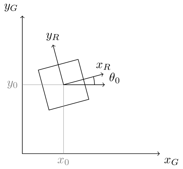
We can refer to the current pose (\(\vec{x}_0\)) of the robot as \(\begin{pmatrix} x_0 \\ y_0 \\ \theta_0 \end{pmatrix}\). This is just fancy notation for a point on the field \((x_0, y_0)\) with a specified orientation of the robot–the heading \(\theta_0\). A pose generally has some beginning origin in the coordinate frame.
Updating the Pose
The change in pose over some very small amount of time is \(\Delta \vec{x}\). The difference in time between the current pose and the last pose should be as small as possible to improve the approximations for the math. Teams should update their robot pose every cycle of their control loop.
Updating the pose is as simple as adding the transformed change to the previous pose where \(\varphi = \Delta\theta\)
The idea of odometry is to use sensor data and math to form an approximation for the robot’s pose over time.
Finding the Change in Position
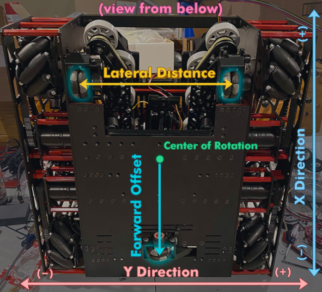
In order to determine the current location of the robot and update its pose, the change must be calculated using data read from the sensors. For a robot, there will be three possible sensors that you can use: two that are parallel with the robot’s body in the \(x\)-direction and one that is aligned with the \(y\)-direction of movement (perpendicular to the drive wheels).
Angle and Displacement
The displacement (or change in position) of the left sensor is \(\Delta x_l\) and the displacement of the right sensor is \(\Delta x_r\). The lateral distance between these two sensors is called the trackwidth, notated as \(L\). This is very important for determining angle for turning approximations. This value will need to be tuned, which means tested repeatedly and then brought to some converging value that is close to the actual measurement.
Deriving the value of \(\varphi\) then becomes simple:
To perform later calculations, we need to know the displacement of the robot in the x-direction relative to its center rather than the two parallel sensors. To do this, we take the average to derive \(\Delta x_c\), or the center displacement:
The final displacement we need before we can determine the change in pose is the horizontal displacement \(\Delta x_\perp\). This is the displacement of the perpendicular sensor \(\Delta x_h\) with a correction for forward offset \(F\). In order to get accurate approximations, the forward offset needs to be considered. When the sensor is closer to the back, the offset is negative, but when it is closer to the front, it is positive. This is to account for the change in its position based on point-turns.
As a result of this, we can define our horizontal displacement as:
Note
If you do not have perpendicular sensors, which are not required if the robot cannot move in the lateral direction, \(\Delta x_\perp\) is not necessary.
For this value, use 0 if you do not have a horizontal sensor.
Robot-Relative Deltas
Let’s come up with a simplified, nonoptimal way to calculate our robot-relative pose deltas which we can then transform into field-relative coordinate changes. To perform this we need to transform the robot-relative deltas via a rotation matrix where we rotate the relative pose difference by the original heading. We can derive the values of \(\Delta x\) and \(\Delta y\).
From this, we can calculate our field-relative change in pose:
Note
This method of approximating position is known as Euler integration, but we are using it for strict pose deltas instead of integrating the velocity (essentially, this is a very simplified version of the original theory).
Warning
This is for advanced programmers; while implementing this from scratch is a great learning exercise, it is likely not the optimal way to get the best auto. There are several resources out there for producing great, well-tested, and easy-to-implement odometry.
Odometry Pseudocode
while robot_is_active():
   delta_left_encoder_pos = left_encoder_pos - prev_left_encoder_pos
   delta_right_encoder_pos = right_encoder_pos - prev_right_encoder_pos
   delta_center_encoder_pos = center_encoder_pos - prev_center_encoder_pos

   phi = (delta_left_encoder_pos - delta_right_encoder_pos) / trackwidth
   delta_middle_pos = (delta_left_encoder_pos + delta_right_encoder_pos) / 2
   delta_perp_pos = delta_center_encoder_pos - forward_offset * phi

   delta_x = delta_middle_pos * cos(heading) - delta_perp_pos * sin(heading)
   delta_y = delta_middle_pos * sin(heading) + delta_perp_pos * cos(heading)

   x_pos += delta_x
   y_pos += delta_y
   heading += phi

   prev_left_encoder_pos = left_encoder_pos
   prev_right_encoder_pos = right_encoder_pos
   prev_center_encoder_pos = center_encoder_pos
Using Pose Exponentials
This method uses differential equations to solve the nonlinear position of the robot given constant curvature. Euler integration assumes that the robot follows a straight path between updates, which can lead to inaccurate approximations when traveling around curves. If you are interested in the math itself, we recommend you check out this book for FRC® controls.
We’ll treat the way it is solved in this page as a black box, and derive the formula by implementing a correction for this nonlinear curvature into our Euler integration robot-relative deltas equation:
Resources for Odometry
There are several great resources out there for odometry. We highly recommend Road Runner. For the math behind Road Runner (which utilizes pose exponentials), you can also read Ryan’s paper. An additional resource for Road Runner is Learn Road Runner which is a step-by-step procedural guide that explains how to work with the Road Runner quickstart.
We also recommend Tyler’s book as it goes into great detail about various controls in FIRST® robotics.
If you’re using other resources, it is important that you do not use ones that utilize Euler integration as it is less optimal for real life approximations of robot pose.